
Question 1) What is the supply curve? What is the demand curve?
The supply curve illustrates the relationship between the quantity of a good that producers are willing to sell and the price of the good. The supply curve slopes upward because the higher the price is, the more that firms are willing to produce and sell. Similarly, the demand curve illustrates the relationship between the quantity of a good that consumers are willing to buy and the price of the good. The demand curve slopes downward because consumers will be inclined to purchase more of a good if the price decreases.
Question 2) Explain the difference between a shift in the supply curve and a movement along the supply curve.
The response of quantity supplied to changes in price are represented by movements along the supply curve itself. So essentially, movements along either the supply and demand curve are the result of changing prices. Shifts of the supply or demand curve are caused by non price related factors such as income or the price of related goods, etc. Movements along a particular curve are referred to as changes in quantity supplied/demanded and shifts of a particular curve are referred to as changes in supply/demand.
Question 3) Define and explain normal goods, inferior goods, complements and substitutes.
A normal good is a good/commodity for which an increase in income leads to an increase in demand. An inferior good is a good for which an increase in income leads to a decrease in demand. Substitutes are two goods for which an increase in the price of one of the goods will lead directly to an increase in demand for the other good. For example, if the price of coffee increases then you may switch your consumption to some other caffeinated drink. Complements are two goods for which an increase in the price of one leads to a decrease in the demand for the other.
Question 4) Define and explain surpluses and shortages and how they relate to price floors and ceilings.
A surplus is a scenario where quantity supplied exceeds quantity demanded. A market may experience a surplus if the government implements a price floor, which is simply a legal mandate preventing prices from falling below a certain level. A shortage is a scenario where quantity demanded exceeds quantity supplied. A market may experience a shortage if the government implements a price ceiling, which is simply a legal mandate preventing prices from rising above a certain level.
Question 5) Explain the process by which one can solve for equilibrium price and quantity. Solve for equilibrium price and quantity in the market model below.
At the introductory level, the method to solve for equilibrium price and quantity is very simple and requires only basic algebra. You will generally be given a demand equation and a supply equation, all you do is set demand equal to supply and solve using either the substitution and elimination method or if the equation turns out to be a quadratic polynomial then you just factor or apply the quadratic formula.
The market model we've been given is taken from Fundamental Methods of Mathematical Economics by Alpha Chiang, 4th edition. #1 page 34.
Qd=Qs
Qd=21-3P
Qs=-4+8P
21-3P=-4+8P (set the supply equation equal to the demand equation)
25-3P=8P (add 4 to both sides)
25=11P (add 3P to both sides)
2.272=P (divide 11 by both sides)
Thus, equilibrium price is equal to $2.272. We can plug in this value into either the Qd or the Qs equation to get equilibrium quantity. We will plug P into the Qd equation.
Qd=21-3(2.272)
Q=21-6.816
Q=14.184
Therefore, for the market model above equilibrium price=$2.272 and equilibrium quantity=14.184.
Question 6) Define the price elasticity of demand and the income elasticity of demand.
The price elasticity of demand measures how much the quantity demanded of a good responds to a change in the price of the good. The price elasticity of demand can be calculated by dividing the percentage change in quantity demanded by the percentage change in the price. The income elasticity of demand measures how much the quantity demanded of a good responds to changes in the consumer's income. The income elasticity of demand can be calculate by dividing the percentage change in quantity demanded by the percentage change in income. As we've already stated, higher income generally results in higher demand since most goods are normal.
Question 7) Define and explain the cross elasticity of demand and the price elasticity of supply.
The cross elasticity of demand measures how much quantity demanded for one good responds to a change in the price of another good. The cross elasticity of demand is calculated by dividing the percentage change in quantity demanded of good 1 by the percentage change in the price of good 2. The cross elasticity is highly dependent on whether or not the two goods are substitutes or complements. The price elasticity of supply measures how much quantity supplied responds to a change in the price of the good. It is calculated as the percentage change in quantity supplied by the percentage change in the price.
Question 8) Explain why the long run price elasticity of supply is larger than the short run elasticity of supply.
In economics you will constantly hear the terms 'short run' and 'long run' come up. When economists, particularly microeconomists, use such terms they are speaking specifically about the inputs of the firm. Specifically, the short run is defined as when at least one of the firms inputs is fixed while the long run is defined as when all inputs of the firm are variable. As a result, the price elasticity of supply in the long run is larger than it is in the short run. In the short run, one or more of the firms inputs may be fixed and as a result it is more difficult for the firm to adjust supply in response to changes in the price. However, in the long run all inputs are variable, not fixed, and as a result firms can easily adjust their supply to match the changing price conditions. Having a larger price elasticity simply means that firms are more apt to respond and change their supply.
Part 2: Consumer Theory 1: Utility and Choice
Some preliminary concepts: Consumer theory is a branch of microeconomics that attempts to model consumer behavior and how consumers go about relating their preferences to the goods they buy and how much of their income to save or spend and etc. At the heart of consumer lies a very fundamental concept known as utility. Utility is simply the amount of satisfaction that an individual derives from consumer a particular good or service. An indifference curve, sometimes called a preference map, is simply a graph that depicts two goods on the horizontal and vertical axis. Within the context of an indifference curve all combinations of the two goods yield the same amount of utility to the consumer, and therefore the consumer is said to be indifferent to different points of consumption so long as these points lie on the same indifference curve.
Question 1) What are the three basic assumptions about individual preferences?
The first assumption is known as the assumption of completeness. Consumer preferences are assumed to be complete in the sense that consumers have a clear idea of what they want and they are cognitively capable of ranking and ordering all of what they want. Under this assumption, consumers will either prefer good A to good B, or good B to good A, or the consumer will be indifferent to both goods. The next assumption is the transitivity assumption. Preferences are assumed to be transitive in the sense that if a consumer prefers good A to good B, and good B to good C then, ultimately, the consumer will also prefer good A to good C. Lastly, and most importantly, consumers will always prefer more to less. This is the non satiation assumption, which states that consumers are never completely satisfied or satiated with what they have, they will always want more.
Question 2) Why can't indifference curves slope upward and why can't indifference curves intersect?
An indifference curve, or a preference map, shows various combinations of two goods to which consumers are totally indifferent. As a result, indifference curves are downward sloping and convex to the origin because if they were positively sloped then the assumption of non satiation would not hold. Similarly, indifference curves cannot intersect, they will always be parallel to one another in two dimensional space because, once again, the assumption of non satiation would be violated. It is also important to note that consumers will always prefer to be on indifference curves that are further away from the origin due to non satiation.
Question 3) What is the marginal rate of substitution?
The marginal rate of substitution is the slope of an indifference curve. It represents the maximum amount of a good that a consumer is willing to give up in order to obtain an additional unit of the other good. For example, if a consumer moves down an indifference curve he will give up some of good Y to attain more of good X and vice versa. The marginal rate of substitution is what measures this.
Question 4) What is the difference between cardinal utility and ordinal utility?
Ordinal utility refers to the ranking and ordering of market baskets, in terms of utility, from most to least preferred. Cardinal utility describes simply describes how much of one market basket is preferred to another. Cardinal utility, unlike ordinal utility, associates numerical values with market values that cannot be arbitrarily changed.
Question 5) Provide detailed explanations of the budget line, the budget set and the budget constraint.

The budget line represents all bundles/baskets of goods that cost exactly m amount of dollars. Whenever an individual is consuming exactly on his budget line he is exhausting all of his income. Therefore, all points on the budget line represent points of consumption that will exactly exhaust the consumers income. The budget set consists of all baskets and bundles that are affordable to the consumer. All points to the left of the budget line, inside the budget set, are affordable while all points to the right of the budget line, outside the budget set, are not affordable to the consumer. This entire graph is called the budget constraint. The mathematics of the budget constraint is as follows:
Px*X + Py*Y =I (the equation states that the total amount spend on good X plus the total amount spend on good Y is equal to the among of income the consumer has).
We will now solve the equation for Y.
Y= -(Px/Py)X + I/Py (this equation essentially says the same thing as the first equation except this equation is now in slope intercept form. The Y intercept of the budget constraint is given by I/Py and the slope is given by -Px/Py.)
Question 6) Explain the process and condition by which utility maximization occurs.

We will now combine our analysis of the budget constraint along with indifference curves to see how utility maximization occurs. In the graph above we have three indifference curves along with a straight budget line with one point that is directly tangent to the green indifference curve. In short, utility maximization occurs at the point where the slope of the budget line is equal to the slope of the indifference curve. This occurs at point A on the graph. At point A, the marginal rate of substitution of good x and good y is equal to the price of x over the price of y. We can write this mathematically as MRSx,y=Px/Py. This is the condition that the consumer must fulfill in order to maximize utility. We can rewrite the condition in terms of marginal utility where MRSx,y=Px/Py => MUx/Px=MUy/Py.
Now, let us assume for a moment that the consumer doesn't initially start off at point A. Suppose the consumer is on the blue indifference curve and is consuming at the point tangent to the budget line above point A on the blue curve. In this case the consumer id deriving more utility from consuming more of good X over the utility being derived from good Y, this can be written as MRSx,y>Px/Py. As a result the consumer will move down the budget line until he reaches point A. At this point the consumer is exhausting his entire in the consumption of the market basket that provides him with the greatest level of utility.
Part 3: Consumer Theory 2: Advanced Topics
Question 1) Explain the substitution and income effects.

In economics, the decrease in the price of a goods will set two effects into motion. The substitution effect is the change in quantity demanded caused by the substitution of one good for another. The income effect is the part of change in quantity demanded caused by a change in real income. From the graph above, let us assume that the price of product B falls. Since the price of product B has fallen both the substitution and income effects will be set into motion. The decrease in the price of product B will induce the consumer to purchase more of B and less of A (assuming that product B is a normal good). Thus, the consumer will move down the indifference curve from Q2 to Q6, the substitution effect is depicted as the movement along an indifference curve. Additionally, the decrease in the price of product B has the effect of increasing the consumer's real income. Since the consumer's real income has increased the budget line will rotate outward and the consumer will be able to attain a higher level of utility on a new indifference curve. In the graph, the income effect is depicted as the move from point Q6 to point Q4. The income effect can be understood as the move to a new indifference curve.
Question 2) Describe what is meant by the labor-leisure trade off. Explain how an individual goes about deciding how much labor to offer and how much leisure to purchase.
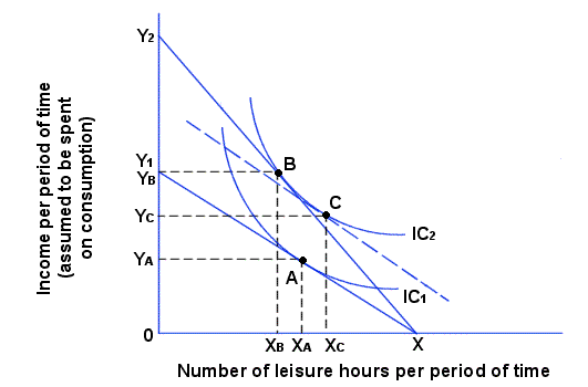
Economists will generally assume that all individuals are faced with two options. First, individuals can choose to work and participate in the labor market and generate income, or they can choose to refrain from working and instead devote their time to leisure, non income generating activities. The labor leisure tradeoff models how individuals decide how much of their time they allocate to either labor of leisure, and the key variable that influences individual's decisions regarding labor and leisure is the wage rate. Holding everything else constant, an increase in the wage rate will induce individuals to offer more labor and purchase less leisure, while a decrease in the wage rate will induce individuals to offer less labor and purchase more leisure.
Now, we will assume that the wage rate increases and apply the substitution and income effects accordingly. As the wage rate increases the opportunity cost of leisure increases and people will be motivated to offer more labor and purchase less leisure. This is the substitution effect because the higher wage rate causes people to substitute labor for leisure. However, the higher wage rate also sets off the income effect which causes people's real income to increase. Since leisure is treated as a normal good, the higher wage rate will motivate consumers to purchase more leisure. As you can see, in the context of labor supply the substitution and income effects work against each other. The substitution effect will move the individual from point A from point B, illustrating the substitution of labor for leisure, however the income effect will move the consumer from point B to point C, illustrating the fact that the increase in income will cause the consumer to purchase more leisure.
Question 3) What is the theory of intertemporal choice? Explain Irving Fischer's model of intertemporal consumption.
Intertemporal choice simply refers to consumption that takes place over different periods of time. In order to answer this question it is crucial that we first understand what savings is. Savings is merely deferred consumption. Whenever you save your money you are merely deferring your consumption to some future time. Therefore, we can break up time into the present and the future or present consumption and future consumption. According to Irving Fischer, the economist who developed this model, intertemporal consumption is ultimately coordinated by the interest rate, which determines how much individuals will want to save. If the interest rate is low than the individual will choose present consumption over future consumption, however, if the interest rate is high the individual will choose future consumption over present consumption.
Let us assume that the interest rate changes. If the interest rate changes then the substitution and income effects will be set into motion. In the context of intertemporal consumption, the substitution effect is always positive, meaning an increase in the interest rate causes present consumption to fall and saving to increase. On the other hand, the income effect is negative meaning an increase in the interest rate will cause present consumption to increase and savings to fall.
Question 4) What is meant by revealed preference? Explain what the weak axiom of revealed preference is and what the strong axiom of revealed preference is.
Recall from part 2, that the preferences of a consumer determine his or her choices and consumption patterns. We are, in a sense, saying that preferences are the key determinant to choices. Now, the concept of revealed preference is merely a reversal of this. Rather than using preferences to determine choices, we will now use consumers choices and purchasing habits to reveal their preferences. Under the idea of revealed preference, choices reveal information about preferences. Essentially, the whole idea of revealed preference was developed as a way to check and validate the underlying assumptions of consumer theory. There is much background knowledge that is required to fully understand the weak and strong axiom of revealed preference.
First, we will discuss how preference can be revealed. Preferences can be revealed directly and indirectly. If a consumer purchases basket X over basket Y, and if both baskets are equally affordable, then the consumer has directly revealed that he prefers X to Y. Preferences can also be revealed indirectly. Suppose that the consumer purchases basket X over basket Y, in this case X is revealed to be directly preferred to Y. The consumer also purchases basket Y over basket Z, therefore Y is revealed to be directly preferred to basket Z. By the assumption of transitivity, we can conclude that basket X is revealed to be indirectly preferred to basket Z. Now that we understand the process by which preferences can be revealed we can now move onto analyzing the weak and strong axiom of revealed preferences.
The weak axiom of revealed preference states that if basket X is revealed to be directly preferred to basket Y then it can never be the case that Y is directly preferred to X. In other words, if Y is affordable and X is purchased then if Y is ever purchased it must be the case that X is not affordable. The strong axiom of revealed preference is basically the same as the weak axiom, except the strong axiom takes into account indirectly revealed preferences while the weak axiom confines itself only to directly revealed preferences.
Question 5) Define and explain the Slutsky equation.
Thus far we have spent an enormous amount of time discussing the substitution and income effects. These two effects play pivotal roles in consumer theory as well as some aspects of producer. Now, what the Slutsky equation does is breaks down these two effects based on uncompensated Marshallian demand and compensated Hicksian demand. Therefore, in order to understand the Slutsky equation we must first understand the difference between Marshallian demand and Hicksian demand.
Recall, from the labor-leisure section, that the substitution and income effects work against one another. Therefore, the total change in change will be the result of whichever effect is the strongest. This is where Marshallian and Hicksian demand comes into play. Uncompensated Marshallian demand simply shows the relationship between price and quantity demanded, however, Hicksian demand shows the relationship between price, quantity demanded and the price of other goods. As such, Marshallian demand reflects the income effect and Hicksian demand reflects the substitution effect.
In order to derive the Slutsky equation we must first take derivatives of the Marshallian and Hicksian demand functions, however we will not do so here. We will merely note that the Slusky equation shows how the total change in demand is equal to the substitution effect minus the income effect.
Part 4: Producer Theory 1: Costs and Profits
Question 1) Explain the difference between diminishing returns and fixed proportions.
The amount of output produced by a firm is determined by the firms production function. A basic production function can be written as Y=F(K,L) where Y=Total Output, K=Capital and L=Labor. The function shows us that output is a function of capital and labor, otherwise known as inputs or factors of production. A production function will either exhibit diminishing returns (also sometimes called variable proportions) or fixed proportions. A firm that has a diminishing returns production function will experience falling output if one input is increased while all other inputs are held constant. If the firm continues to increase the amount of the factor input then, eventually, the factor input will begin generating diminishing returns for the firm. A fixed proportions production function requires fixed amounts of inputs to be used at all times. Meaning, if the firm wishes to produce some level of output then it must employ a fixed and constant level of inputs. The firm cannot arbitrarily change the amount of capital and labor used, instead the firm is forced to use capital and labor in fixed proportions.
In the primary/agricultural sector of the economy diminishing returns generally dominates because as more workers are hired to work the land and operate the capital then overall returns begin to diminish. Workers, being a variable input, are being added to land, a fixed input, and as a result the marginal product being generated by workers will begin to decline as more workers are hired. On the other hand, fixed proportions dominates the secondary/manufacturing sector of the economy. For example, if the only way a manufacturer can produce a chair is with 1 unit of labor and 3 units of capital, and the manufacturer has 2 units of labor and 5 units of capital, then 1 unit of labor and 2 units of capital will remain idle.
Question 2) What is fixed cost, variable cost, average fixed cost, average variable cost, average total cost and marginal cost? Derive cost and revenue functions from the given the market model below.
Fixed costs are costs that are incurred by a firm regardless of the scale of output. The firm could be producing absolutely nothing at all and yet, the firm would still have to pay fixed costs. Variable costs are costs that vary directly with the scale of production. If the firm is producing zero output then the firm will have to pay zero variable costs. However, as the scale of production increases then variable costs will increase as well. Average fixed cost and average variable cost is simple fixed and variable costs divided by quantity. Total cost is simply fixed cost plus variable cost and average total cost is total cost divided quantity. Now, whenever we see the word 'marginal' in economics we want to automatically associate that word with change. Marginal cost is the change in total cost divided by the change in quantity.
In the market model below, 1) derive the marginal revenue function from the given total revenue function 2) derive the variable cost function from the given total cost function 3) derive the marginal cost function from the given average cost function.
-Total Revenue: 15Q - Q^2
-Marginal Revenue: 15 - 2Q (In order to obtain a marginal revenue function from a total revenue function all we do is differentiate the total revenue function.)
-Total Cost: Q^3 - 5Q^2 + 12Q + 75
-Variable Cost: Q^3 -5Q^2 + 12Q (In order to derive variable cost from total cost all we do is eliminate any constant that doesn't have a Q attached to it. This is because variable cost is attached to quantity while fixed cost isn't. Any constant by itself is fixed cost and can thus be eliminated in order to attain a variable cost function.)
-Average Cost: Q^2 - 4Q +174
-Total Cost: Q^3 - 4Q^2 +174Q (We cannot derive marginal cost directly from average cost. We must first find the original total cost function, which can be found by multiplying the average cost function by Q.)
-Marginal Cost: 3Q^2 - 4Q +174 (Marginal cost is the derivative of total cost.)
Question 3) Draw and explain the unit cost structure for a firm experiencing diminishing returns.
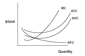
At first glance the graph above can look quite intimidating. But, the graph merely provides a visual representation for everything that was written in the answer to question 2 of the section. We will first look at average fixed cost and average variable cost. When the firm is producing zero output then the firm is only paying its average fixed cost and the AFC curve extends upwards indefinitely. However, as the firm begins to produce some quantity of output then average variable cost comes into play. AFC begins to shrink because the fixed costs are spread over a wider quantity of production and AVC begins to increase because the higher levels of production bring about higher variable costs. Thus, the graph shows that at very low output levels fixed costs dominate but when quantity produced increases variable costs dominate and fixed costs shrink.
Now we will look at the relationship between average total cost and average fixed cost. First, average total cost reflects both average fixed cost and average variable cost and this is seen in the shape of the ATC curve. Marginal cost is the change in total cost divided by the change in quantity, and as a result the MC curve will ALWAYS intersect the ATC curve at its LOWEST POINT. Whenever marginal cost is below the ATC curve, average total cost is falling. Similarly, whenever marginal cost is above the ATC curve, average total cost is rising. Why is this? Average total cost represents cumulative output while marginal cost represents the change in output. If the change in output is high then obviously the overall/cumulative level of output will also be high. If the change in output is small then obviously the overall/cumulative level of output will also be small.
Question 4) Explain the unit cost structure for a firm experiencing fixed proportions.
As we already stated, under the case of fixed proportions inputs must be used in a fixed ratio to one another. As such, if a production function exhibits fixed proportions labor and capital can never be changed. They must always remain constant. The key thing to remember is that under the case of fixed proportions average variable cost is always equal to marginal cost. This is because any change in output will cause all inputs to change at an equal rate, which in turn will cause all costs of inputs to increase in equal rates as well.
Question 5) What is the rule of profit maximization that all firms must follow?
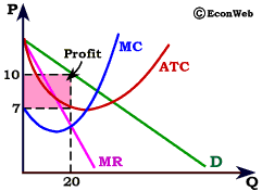
A firms profits will always be at its maximum level where marginal revenue is equal to marginal cost, or MR=MC. Remember, profits are equal to revenue minus costs. The larger the gap between total revenue and total cost then the larger the firms profits will be. Again, this is captured by the equation MR=MC. If MR exceeds MC then the firm should increase production in order to equilibrate the two. If MR is below MC then the firm should decrease production in order to equilibrate the two. The above graph provides a visual depiction of the profit maximization rule.
We have taken the typical unit cost structure for a firm experiencing diminishing returns and we've drawn in a linear demand curve and linear marginal revenue curve. We will simply observe wherever the MR curve intersects the MC curve and at that point we will draw a vertical line upwards right until the line hits the demand curve. At this point the firm will maximize profits by producing 20 units of output at a price of 10 dollars. This rule of profit maximization applies to all firms regardless of whether they're monopolists or oligopolists or perfectly competitive firms.
Question 6) Under what conditions will a firm shut down? Under what conditions will a firm breakeven? Under what conditions will a firm exist the market?
The firm will implement a shutdown of production the revenue being generated cannot cover the variable costs of production. This means that as the firm produces more then the firm will incur costs that will exceed the amount of revenue its getting. Thus, the shutdown rule can be written as TR < VC where total revenue is less than variable costs. A shutdown occurs in the short run while an exist occurs in the long run. This is because in the short run fixed costs are unavoidable while in the long run fixed costs do not exist. Remember, even if the firm produces nothing it will still have to pay fixed costs so a shutdown of production won't eliminate fixed costs. The firm can only rid itself of fixed costs if it completely exists the markets. Therefore, the exist rule can be written as TR <TC where total revenue is less than total cost, where total cost is the sum of fixed and variable cost. The breakeven point occurs when the level of output generates enough revenue to cover all the firms costs. If the firm is below the breakeven point then it is generating losses, if the firm is above the breakeven point then it is generating profits.
Part 5: Producer Theory 2: Advanced Topics
Question 1) What are isoquants and isocosts?
Recall that from consumer theory we had these things called indifference curves, and any point on one single indifference curve represented different combinations of two different goods that provide the same level of utility to the consumer. Isoquants are pretty much the same thing, except with isoquants we're dealing with producers, not consumers. An isoquant is a curve, shaped the same way as an indifference curve is, and any point on the isoquant represents different combinations of capital and labor that yield the same level of output. Now, the isocost line is basically the same as the budget line from consumer theory. An isocost line is a straight, linear curve that slopes downward from the vertical to the horizontal axis. The isocost line represents all combinations of capital and labor that cost the same. Therefore, when the firm is producing on a particular isocost line then all input are cost equivalent. Given an isocost line, the firm can produce at all points to the left of the line or on the line itself. Points to the right of the isocost represent unattainable levels of production given the firms current technology.
Question 2) What is the marginal rate of technical substitution?
The marginal rate of technical substitution is the slope of the isoquant line. It represents the amount by which one input can be reduced when one more unit of another input is added. Like the marginal rate of substitution for indifference curves, the marginal rate of technical substitution for isoquants is also always negative. It can be written mathematically as MRTS(L,K)= MPL/MPK which stands for the marginal rate of technical substitution for labor and capital is equal to the marginal price of labor over the marginal price of capital.
Question 3) Explain the process of cost minimization. What is the least cost choice of capital and labor for a firm producing some level of output?
We will now combine our understanding of isoquants, isocosts and the marginal rate of technical substitution to explain how the firm goes about minimizing its costs. The process is nearly identical to the process by which consumers maximize utility.

In order to successfully minimize its costs, the firm must find that one point of production where the marginal rate of technical substitution is equal to the marginal price of labor over the marginal price of capital. This is depicted graphically as the point of tangency between the isocost line and the isoquant curve. At the red point on the graph the slope of the isoquant equals the slope of the isocost, and therefore at that point all costs are at their lowest minimum. Now, let us suppose that the firm starts out by producing at the top of the isoquant that intersects the light blue isocost. In this case, the firm has chosen a combination of capital and labor where the marginal rate of technical substitution is greater than the marginal price of labor and capital. At this point the firm is paying its labor a little bit more than it is paying its capital. The firm would be motivated to move down the isoquant curve because it would still maintain the same level of output except at a lower cost. As a result, the firm moves down the isoquant but as it does so the isocost lines shifts inward and this process continues until equilibrium is achieved between the marginal rate of technical substitution and the marginal price of labor and capital.
Question 4) What is the expansion path of a firm?

The expansion path consists of the set of all cost minimizing input combinations a firm will choose to produce output with. To put it more simply, the expansion path is just the curve that passes through all the points of tangency between a firms isocost line and isoquant curves. It tells us the combinations of labor and capital that the firm will choose to minimize costs at with each different output level. In the graph above we're presented with a curvilinear expansion path line. We have three cost minimizing points in the diagram, and the expansion path runs through each of the three points. If the firm wishes to expand or roll back production it should stay on the expansion path in order to ensure that costs are always are their minimum.
Question 5) What is the difference between short run and long run average total costs?

As we have already stated, the short run and the long run are differentiated by fixed and variable inputs. The short run is defined as when at least one of the firms inputs is fixed while the long run is defined as when all inputs of the firm are variable. Because of this, the average total cost curve, which is simply the sum of average fixed and average variable cost, is different in the short run than it is in the long run. The graph above shows how short run ATC is related with long run ATC. The long run ATC curve is much more flatter than any three of the short run ATC curves are and the short run ATC curves all lie above the long run ATC curve. This is primarily due to the fact that in the long run firms have greater freedom and flexibility. Now, the key thing to remember about this graph is that when the long run ATC curve is falling, economies of scale apply. Economies of scale is simply defined as the decline in long run average total cost as the quantity of output increase. It is the cost benefits a firm gets when they grow. When the long run ATC curve is horizontal, constant returns to scale apply, meaning that long run average total cost remains constant as output increases. When the long run ATC curve is rising diseconomies of scale apply. Diseconomies of scale is simply the reverse of economies of scale, it is where long run average total cost increases as output increases.
Question 6) Draw an isoquant diagram for a firm experiencing fixed proportions.
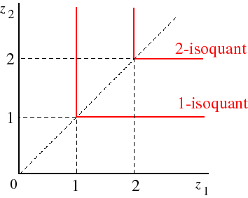
The above graph is an isoquant map for a firm experiencing fixed proportions. As we've already said, under the case of fixed proportions inputs must be used in a fixed ratio to one another. As such, if a production function exhibits fixed proportions labor and capital can never be changed. Notice that in this particular diagram, the firms isoquants are L shaped, they are not convex to the origin unlike the other isoquants we've been dealing with. This is because, on the vertical and horizontal segments of the L shaped isoquant, either the marginal product of capital or the marginal product of labor is zero. If the firm wishes to move up the expansion path and increase production then the firm must increase labor and capital jointly. In this case higher levels of output can only be realized when both labor and capital are added in fixed proportions.
Part 6: Market Structures
Question 1) What are the key characteristics of perfectly competitive markets? What is the long run outcome of perfectly competitive markets?
A perfectly competitive market structure exists when any particular market is dominated by a large number of sellers. As such, every single firm in the market will be a price taker, meaning that they will have no power to control or alter the price of their product. They will be at the mercy of the market, and they must take the price given by the competitive conditions of the market. Additionally, perfectly competitive markets will have virtually no barriers to entry, allowing firms to enter and exist as they please and the product in the market must be homogenous. The long run outcome of a perfectly competitive market is that each firm will only make accounting profits. In other words, firms in a perfectly competitive market structure will make no economic profits in the long run.
We will now explain the difference between accounting and economic profits. Accounting profits (also called explicit or normal profits) are the profits a firm generates by subtracting total revenue from total cost. These profits can be explicitly recorded in the firms financial statements. Economic profits (implicit profits or supernormal profits) not only takes into account total cost, but also the opportunity costs of owning and running a business. Again, the opportunity cost of running your own business is whatever else you could've done instead. Supernormal profits cannot be earned under competitive market structures in the long run because if any single firm does begin earning above normal profits, capitalists will invade the market and profits will eventually be pushed back down to their normal levels.
Question 2) What is a monopoly? Explain the profit maximizing choice of a monopolist.

A monopoly is a type of market structure that is dominated by only one firm. The main reason why monopolies come into existence is due to barriers to entry that make it harder for other capitalists to come into the market and set up shop. The monopolist will maximize profits in the same way all other firms maximize profits, and that is by finding the appropriate output level where Marginal Revenue=Marginal Cost. However, the difference between monopolies and perfectly competitive firms is that with perfectly competitive firms, the price being charge must also equal the firms marginal revenue and marginal cost. The perfectly competitive firm is a price taker and must take the going market price. However, monopolies are price setters. Monopolist have the ability to change their prices at will and can increase prices above marginal revenue and marginal cost.
Therefore, a perfectly competitive firm's price=marginal revenue=marginal cost whereas a monopolist's price>marginal revenue=marginal cost. Thus, the monopolist firm will maximize profits by restricting supply, causing prices to rise it will generate supernormal profits as a result. Monopolies are not hugely undesirable because they essentially impose an unwarranted tax on society by forcing consumers to pay a price that far exceeds the unit costs of production.
Question 3) What is an oligopoly? Use the theory of the kinked demand curve to explain oligopolistic market structures.

The basic idea underscoring the theory of oligopoly is that it consists of a market structure dominated by a handful of firms with enormous economic power. Because there's such a small number of large firms, there's constant pressure on each firm to be attentive to the behavior of other firms in the market. An outcome that is common of oligopolistic markets is that prices tend to remain fairly constant in the long run. Oligopolies are considered inefficiency by social welfare standards because when the collude with one another they are essentially acting as a monopoly would and they produce all the same inefficient effects that monopolies produce, namely restricting supply and keeping prices abnormally high.
The kinked demand curve provides a visual depiction for the pricing behavior of oligopolies. The cost structure above represents the cost condition of an average oligopolist. The key idea that the graph captures is that at equilibrium price and quantity (denoted by point A in the graph) the oligopolist is convinced that if he raises his price the other firms will hold onto theirs. Each firm is convinced that the demand for its product is very elastic above the equilibrium point. At the same time, each firm is also convinced that if they lower their price the other firms will immediately follow, meaning each firm is convinced that demand for its product is inelastic below the existing price. As a result of this the marginal revenue curve is kinked, along with the demand curve. The kinked demand curve helps explain why it is that oligopolists hold onto existing prices for quite some tie despite changing cost conditions.
Question 4) What is monopolistic competition? What is the long run outcome of monopolistically competitive firms?
Monopolistic competition is a type of market structure where there are many firms selling products that are similar but not identical. The products sold in monopolistically competitive markets are differentiated, but only slightly. Now, the problem with monopolistically competitive markets is that within these markets there are too many firms producing and supplying the similar products. So, the long run outcome of monopolistically competitive markets is that the firms within these markets operate with excess capacity.
Question 5) Define and explain the Cournot model and Nash equilibrium.
The Cournot model of competition and equilibrium represents a field of study known as game theory, which has many applications in economics. Within the context of game theory and the Cournot model we are analyzing the behavior and decisions of different actors in a given situation and how these actors will respond to one another. There are three main factors that are central to game theory. We have the players in the game, we have the actions of each player and lastly, we have the payoffs to each player subject to their actions. In the case of the Cournot model the players are the different firms in the market, the actions of the firms are the possible levels of output they will supply, and the payoffs to each firm are, of course, their profits.
Now, the Cournot model rests on the main assumption that firms in an oligopolistic market will compete with each other. However, we know that in reality this may not happen because collusion is very common among oligopolies and the firms may get together and form a cartel. Given this collusion the Cournot model doesn't apply and we can toss it out the window. However, if we are presented with an oligopolistic market structure where the firms are competing then this model provides very useful insights. Oligopolistic firms cannot compete the way traditional firms can, which is by lowering the price and the kinked demand curve explains why. Since price is not the motivating factor here, what other factor besides price can firms compete on? The answer is the quantity of output or the amount of goods they sell. Firms will react to one another based on what they believe is the amount the other firm will produce. This is idea captured in a reaction function:
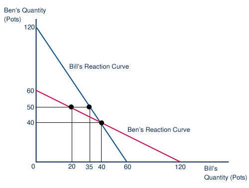
Let us assume that we have a two firm market, a duopoly, that consists of Bill's shop and Ben's shop. Both of these firms sell identical products, pots, and both firms are competing with each other. As we can already see, equilibrium in the Cournot model is achieved when both firms reaction curves intersect. Now, this is the way the reaction curves work. Ben's profit maximizing output is a decreasing schedule of how much he believes Bill will produce. Meaning, the more the Bill produces the less that Ben will produce. Look at the graph, if Bill produces 0 output 60 units of output, if Bill produces 20 Ben will decrease his output production to 50 and if Bill increases his output all the way to 100 Ben will react by producing 0 output. The same is true for Bill. Now, like we already said equilibrium in the model occurs at the intersection of Bill's and Ben's reaction curves. At the equilibrium point both Ben and Bill have correctly guessed the output levels of their counterparts and have adjusted their production accordingly. This is called a Nash equilibrium because both players in the game have correctly anticipated the others actions.
Question 6) What is a monopsony? Draw and explain the profit maximizing choice of labor for a monopsonistic firm.
Economists will delineate between input markets and output markets. Output markets are just typical every markets where consumers buy goods from producers. Input markets are markets where producers buy factors of productions (or inputs) from consumers. The labor market is an example of an input market because businesses are buying labor from consumers. Monopolies exist in the output market, and we already know what a monopoly is. A monopsony is the same thing as a monopoly, except monopsony's exist in the input market. In general, a monopsony is a type of market structure where there is only buyer but many sellers. This is the equivalent of having one business in a small town and many job applicants.

The following graph depicts a monopsonist intent on hiring the profit maximizing amount of labor. The monopsonist will pick that usage of labor that will insure that the marginal revenue product of labor is equal to the marginal cost of labor. In the graph this occurs at the point where the MRP curves meets the MC curve. The thing to note about this choice is that the monopsonist will always pay it's workers less than what would be paid in a competitive labor market while, at the same time, hiring less workers than what would be hired in a competitive labor market.
Part 7: General Equilibrium Theory and Welfare Economics
Some preliminary concepts: The whole idea of general equilibrium can be contrasted with the idea behind partial equilibrium. We already know what partial equilibrium is, we discussed it in the very first section. Partial equilibrium in a market occurs where supply meets demand, and from there we can derive an equilibrium price and quantity. Now, many economists over the years have postulated a general equilibrium whereby an equilibrium price and quantity emerge for all markets in the economy simultaneously. This was, for me personally, the most challenging topic in all of economics. The material can be very esoteric and abstract at some points, and additionally, the entire theory of general equilibrium should be approached very skeptically. Many economists, include Milton Friedman above all else, have been somewhat critical of the theory due to the many precise and rigorous assumptions it requires. The theory is a work of art that makes much sense and provides much much insight, but it doesn't offer much in terms of usefulness and practicality.
Question 1) Explain what is meant by pareto optimality? What is a pareto optimal allocation of goods?
Pareto optimality, named after an economist by the name of Vilfredo Pareto, states that maximum welfare occurs when there is a situation where you cannot make someone better off without making someone else worse off. Under this condition, all goods are allocated in such a way that a change in the allocation will cause overall welfare to diminish. The pareto optimal allocation of goods that maximizes total consumer welfare when all actors in the economy have identical marginal rates of substitution. To make things simple, we will assume a two person economy and show how a pareto optimal allocation may take place. If we have two people in an economy, and the initial allocation of goods is not optimal, then obviously these two people will trade and exchange their goods with one another until they get what they desire. The exchange and the trade will end once both consumers are satisfied and there are no further possibilities for an exchange that will make at least one of them better off. At this point, the marginal rate of substitution for both individuals is equal and all goods have been allocated in a pareto optimal way.
Question 2) Explain in detail the components of the Edgeworth box.
The Edgeworth box is simply a diagram that illustrates everything that was said in the answer to the first question, it provides a visual representation for how a pareto optimal allocation of goods occurs.
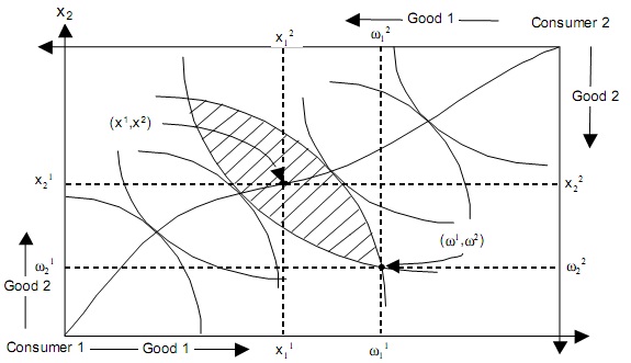
In the Edgeworth box we are assuming that there are only 2 consumers in the entire economy. All points within the box represent some possible allocation of goods between the two consumers and our goal is to determine which of the allocations offer mutually beneficial trades to both the consumers. The initial allocation of goods is at (w1,w2), and consumer 1 and consumer 2's indifference curves have been drawn into the box. The way to tell which indifference curve belongs to which consumer is to look at which way they are directed. All indifference curves which are convex to the corner where consumer 1 is belong to consumer 1, and the same is true for consumer 2. Now, like we already said, the initial allocation of goods is shown by the point (w1,w2). The curvilinear line that runs through the box diagonally is known as the contract curve, it represents all allocations of goods that are pareto optimal. We do not know what the ultimate allocation of goods will be between these two consumers, but we do know that in order for a pareto optimum to occur the consumer must move to some point on the contract curve. Any point off the contract curve will not be optimal because mutually beneficial trade will still be possible. Now, why do the points on the contract curve represent a pareto optimum? Because all those points lie directly where consumer 1 and consumer 2's indifference curve are tangent to one another. At the point of tangency the marginal rate of substitution for consumer 1 is equal to the marginal rate of substitution for consumer 2, which satisfies the condition for a pareto optimum.
Question 3) What is meant by efficiency in production?
Thus far we have only analyzed the conditions for pareto optimality and efficiency when it comes to consumer trade and exchange. We will now expand our analysis to include not only consumer exchange, but also production. We will later use the production possibilities frontier diagram to illustrate how efficiency in output may take place, just as we used an Edgeworth box diagram to show how efficiency in exchange takes place. First, we will discuss the concept of technical efficiency. Technical efficiency is simply when producers use their inputs in the most efficiency and productive way possible to produce output least expensively. In order for capital and labor to be used in the most efficiency manner the marginal rate of technical substitution for capital must equal the marginal rate of technical substitution for labor. If both marginal rates of technical substitution are equal then there is no possible rearrangement of capital and labor that will make the firm better off. Firms are now using the most efficient least cost combination of labor and capital. This is one of the underlying tenants behind efficiency in exchange., ie minimizing cost. Now, firms must also maximize profits. Firms maximize profits by producing what consumers want. Therefore, the last component of general equilibrium is efficiency in output. Output is considered to be efficient if the marginal rate of substitution for each consumer equals the marginal rate of transformation for each good. We have yet to discuss the marginal rate of transformation. We will now do so in the next question.
Question 4) What is the marginal rate of transformation? Use the Production Possibilities Frontier to illustrate how efficiency in output may occur.
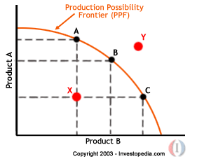
The production possibilities frontier diagram shows all the possible goods an economy can produce. In the graph above, only two possible goods are able to be produced: product A and product B. Now, notice that if we devote all resources into producing A we will get zero amounts of product B, and vice versa. Thus, in order to get some of product A we must forego some of product B, and in order to get some of product B we must forego some of product A. Points A, B and C represent all technically efficient levels of production, point X represents an inefficient level of production because it is possible for more of both A and B to be produced. Typically, any point below the PPF curve can be seen as a recession. Point Y represents some unattainable level of production given the economies current technology. Point Y can be reached if the PPF curve shifts outward. An outward shift of the PPF curve represents economic growth and technological progress.
The marginal rate of transformation is the slope of the PPF curve. It measures how much of product A was given up to produce more of product B, and vice versa. Now, coming back to our discussion of general equilibrium, efficiency in output occurs where the marginal rate of substitution equals the marginal rate of transformation. Under this scenario, the MRT (which measures the cost of producing one goods relative to another) equals the MRS (which measures the marginal benefit of consuming one good relative to another).
Question 5) Explain what is meant by general equilibrium. What are the factors that prevent a general competitive equilibrium.
Now that we have completed our discussion of the components of general equilibrium, we're now more equipped to provide a better explanation for what generally equilibrium actually is. Under general equilibrium, the economy is experiencing efficiency in exchange, production and output. This simply means that all consumers are maximizing utility, all firms are minimizing costs and using inputs in the most technically efficient way and all firms are maximizing profits by providing the appropriate amount and type of output to consumers. Since the allocation of goods and resources under general equilibrium is such as everybody is maximizing everything, it would be impossible to rearrange the allocation of goods or resources without making somebody worse off. Thus, the state of general equilibrium is also a pareto optimum.
Now, there are a few factors that impede a general competitive equilibrium from emerging.. The first thing that must be true is that all markets are perfectly competitive or close to being perfectly competitive. Imperfect competition, such as monopolies, oligopolies, etc, must be non-existent in order for a general equilibrium to arise. The last two factors include externalities and public goods, which will be discussed later on.
Question 6) What are the first and second theorems of welfare economics? Explain Arrow's Impossibility Theorem and the Arrow-Debreu Model.
The first theorem of welfare economics is a key theorem that is essentially a more formal and mathematical restatement of Adam Smith's invisible hand conjecture. The theorem states that if we have a perfectly competitive economy then we will also reach a pareto optimum, even if all the actors in the economy are selfish and greedy. In other words, every general equilibrium is also pareto optimal, we already explained why in question 5. Adam Smith similarly said that the market, through the invisible hand, will guide society towards desirable outcomes (a pareto optimum) even if everyone is greedy and self interested. The second welfare theorem is simply the converse of the first. A pareto optimum can be achieved by a one time governmental redistribution of wealth and then allowing the free market to coordinate exchange from there. Both of these theorems have been mathematically proven.
The Arrow-Debreu model is a key piece of information that lies at the heart of general equilibrium theory. We already know what it is, but now we need to connect the dots. The model tells us that there exists some set of prices that will bring about a general equilibrium whereby supply equates demand in all markets. We already knew this to be the case though so this model is nothing profound. Now, Arrow's impossibility theorem applies economics analysis to politics and voting in particular. The theorem tells us that there is no such political system for aggregating individual preferences into a set of social preference. To make it simpler, Arrow posits 4 criteria that an ideal society would like:
-Unanimity: If everyone wants A rather than B then everyone should get A rather than B
-Transitivity: If A beats B, and B beats C then A should beat C
-No dictators: There is no one person who has all the power
Arrows Impossibility Theorem tells us that there exists no such voting system that can satisfy all these criteria. Arrow's theorem has also been mathematically proven.
Question 7) Explain what a social welfare function is and explain the process and condition by which social welfare can be maximized.
There are several ways by which economists define social welfare. A very simple and crude way to measure social welfare is to add the total amount of consumer and producer surplus in the economy, and by adding these two variables you get your total amount of social welfare. We have not discussed what consumer and producer surplus is and we are not going to because this is a very crude and simplistic way to define social welfare.
A better, more comprehensive way to measure social welfare is with a basic social welfare function. Verbally, a social welfare function shows that social welfare is a function of the summation of all individual utility functions in the society. This can be written mathematically using sigma notation but I'm not capable of producing the exact mathematical function on here. Knowing the verbal definition is sufficient. And once again, you can measure the social welfare of a society by taking the utility of each individual and adding them all together. This is the social welfare function, where social welfare is a function of all the utility in the society. This is hardly a scientific concept though because we are not capable of sticking little chips into people's brains to get the exact level of utility for each person, and as a result the concept of social welfare overall is based on opinion and conjecture as opposed to data and mathematics.
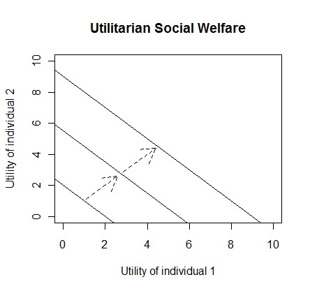
The graph above represents the basic utilitarian social welfare function. On the horizontal axis we are measuring the utility of individual 1 and on the vertical axis we are measuring the utility of individual 2. What the diagram is trying to convey is the idea of tradeoffs between people. The straight lines in the graph represent indifference curves, and each point on the indifference curve represents combinations of utility between individual 1 and 2 to which the entire society is indifferent. If we move up any of the curve individual 2 is better off than individual 1, if we move down any individual curve individual 1 is better off than individual 2. Now, the question becomes one of social welfare maximization? How do we maximize the total amount of social welfare in the entire society? Several theories attempt to answer this question.
From the utilitarian perspective, social welfare can be maximized if wealth and income is transferred from those who place a low value on it to those who place a high value on it. For example, if Warren buffet lost a dollar his overall utility wouldn't diminish by that much because he has billions of them. However, if a homeless person gained a dollar his utility would increase by a lot because he virtually has nothing. Therefore, according to this utilitarian perspective, society should redistribute wealth and income until everybody's marginal utility is equal. Remember, marginal utility is simply the change in utility, and from the example above Buffet's marginal utility wouldn't change by that much if he lost a dollar but the homeless guy's marginal utility would increase by a lot.
The Rawlsian social welfare function states that social welfare can be maximized if we maximize the utility of those in society who are worse off. Unlike the utilitarian social welfare function the Rawlsian social welfare function states that social welfare is a function of the level of minimum utility in the society. As a result, social welfare can be maximized indefinitely if we increase the utility of those worse off members. Mathematically, the function can be written as SW=min(Ui) where SW=Social Welfare, min=minimum and Ui=Utility of each individual. Both the Rawlsian and utilitarian social welfare function viol
